library(ggraph)
library(tidygraph)

gr <- sfnetworks::as_sfnetwork(sfnetworks::roxel)

ggraph(gr, 'sf') +
  geom_edge_sf(aes(color = type)) +
  geom_node_sf(size = 0.3)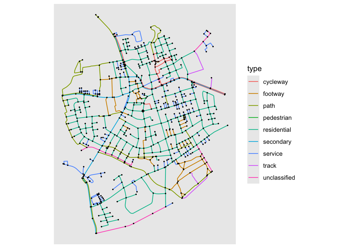
My return to ggraph development was not supposed to end out with something deserving of a blog post. It was supposed to be a quick triage of bugs to quench my bad conscience for not having looked at the package for quite some time (well, the instigator was the new ggplot2 release which required some changes in ggraph). Yet, one thing lead to another and now I’m sitting here, writing a release post indicating that it turned out to be more than just a series of bug fixes.
So, while this is certainly not a monumental release, let’s celebrate the fact that some very welcome additions managed to lure me into a proper update of the package.
What is ggraph? If you came to this blog post not knowing what this is all about (and made it past the two rambling top paragraphs) you have shown an impressive tenacity towards my R package work. ggraph is a ggplot2 extension for visualising relational data (networks, graph, hierarchies, etc.). It is one of the most versatile frameworks for creating network visualisation and all around a great package. You can learn more about it on it’s webpage, which also includes extensive documentation of it’s features.
If the above is old news to you you are probably sitting patiently waiting for me to tell you what is inside this new release. Wait no more…
Some time ago sfnetworks was developed on top of tidygraph to handle spatial network with the tidygraph API. Thanks to a PR from Lorena Crespo ggraph now works natively with this class. The layout itself is pretty simple as it takes the node location already stored in the object and uses them as is. But the layout is also accompanied by a new node and a new edge geom that ensures that the correct CRS is used during plotting etc. The basic use goes something like this:
library(ggraph)
library(tidygraph)
gr <- sfnetworks::as_sfnetwork(sfnetworks::roxel)
ggraph(gr, 'sf') +
geom_edge_sf(aes(color = type)) +
geom_node_sf(size = 0.3)
This can of course be used together with other sf layers for decorations and such (e.g. city boundaries) using geom_sf() from ggplot2.
While you are often going for as correct a representation of the location data as possible when working with spatial data, there are situations where a more stylized look is wanted. One such situation is for railroad and metro maps where the standard has long been to prefer legibility over correctness. ggraph now has a layout that places nodes in a manner akin to what we expect for these types of maps. It is, as many of the layouts in ggraph, provided through the graphlayouts package by David Schoch and, while it is a bit finicky, it can provide a great starting point for a grid-like graph layout.
gr <- as_tbl_graph(graphlayouts::metro_berlin) |>
  convert(to_simple)

ggraph(gr, 'metro', y = lat, x = lon, grid_space = 0.005) +
  geom_edge_link(width = 1) +
  geom_node_point(size = 2) +
  geom_node_point(size = 0.5, color = 'white') +
  coord_fixed()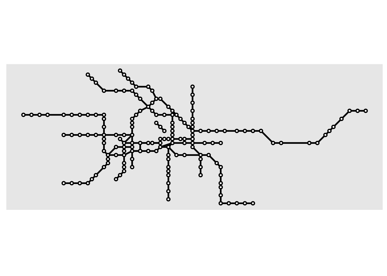
ggraph already has ample of layout choices if your data is hierarchical, and now you are spoiled for even more.
Cactustree is a layout that, if you squint your eyes and are a bit imaginative, resembles a cactus. While that sounds a bit odd at first, it makes pretty good sense once you see it. The layout was developed with hierarchical edge bundling in mind, so while it can certainly be used to show hierarchical relations there are probably better layouts for that if that is your only concern.
gr <- tbl_graph(flare$vertices, flare$edges) |>
  mutate(class = stringr::str_match(name, "flare\\.(\\w+)")[,2])
from <- match(flare$imports$from, flare$vertices$name)
to <- match(flare$imports$to, flare$vertices$name)

ggraph(gr, 'cactustree', scale_factor = 0.5) +
  geom_node_circle(aes(fill = class), colour = NA, alpha = 0.3, show.legend = FALSE) +
  geom_conn_bundle(aes(alpha = after_stat(index)), data = get_con(from, to)) +
  scale_edge_alpha(range = c(0.1, 0.5), guide = 'none') +
  coord_fixed()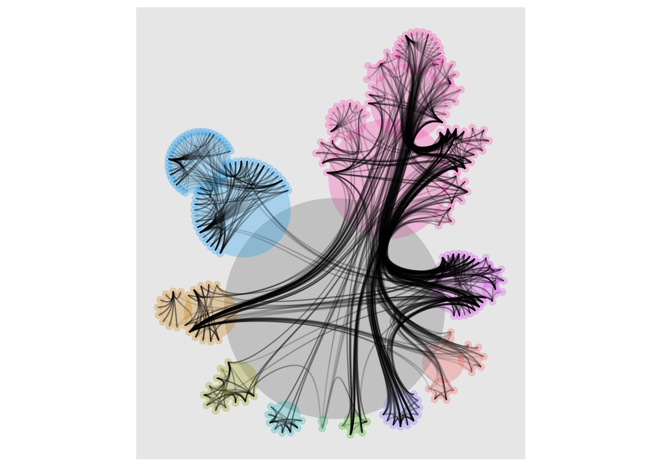
While the above layout is certainly flashy, the next one is not. The H tree layout is a space filling layout that can only be used for binary trees, so it’s application is quite limited. But, if you have a binary tree you need to show, this is your friend:
gr <- create_tree(1023, 2)

ggraph(gr, "htree") +
  geom_edge_link() +
  geom_node_point(aes(filter = leaf))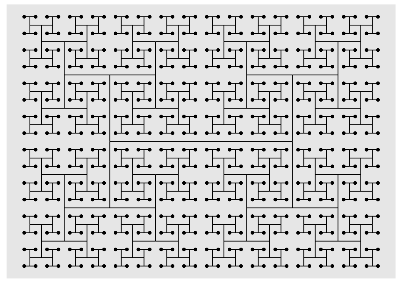
Some of the existing layouts have been updated with new features, worthy of a mention.
The linear layout now has a weight argument that can control the spacing between points. In conjunction with now outputting enough information for use with rect and arc nodes this opens up for some new possibilities
gr <- create_notable('Meredith') |>
  convert(to_directed) |>
  mutate(class = sample(letters[1:6], n(), replace = TRUE),
         size = pmax(0.1, 2 + rnorm(n())),
         amount = runif(n()))

ggraph(gr, "linear", circular = TRUE, weight = size) +
  geom_edge_arc() +
  geom_node_arc_bar(aes(r = 1 + amount/10, fill = class)) +
  coord_fixed()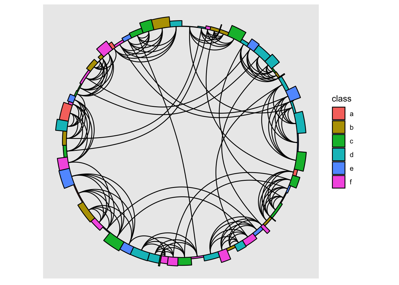
The other updates comes courtesy of new functionality in the graphlayouts package and brings the layouts provided by ggraph up to speed with the implementations in graphlayouts. This means that the focus and centrality layout gets a group argument that allows grouping of kindled nodes in these two layouts. Further, the stress layout (the default layout in ggraph) gains an x and y argument which can be used to fix some (or all) nodes in one or two dimensions. If either is given then NA values indicates that a node should be placed by the layout algorithm, given the constraints of the fixed nodes.
We talked about hierarchical edge bundling back when I showed the cactustree layout. While that was the first (I believe) type of edge bundling it did suffer from the fact that it needed an underlying hierarchical structure for the bundles to work. This created a disconnect between the graph the layout was created on and the edges that was shown (which is why they are drawn with geom_conn_*() not geom_edge_*() functions) that has later been sought to remove. This has created a bunch of different generalised edge bundling techniques and ggraph now supports a few thanks mainly to David Schoch (again).
The force bundling techniques treats edges as springs that attract each other if they run in parallel (it’s a bit more involved but that is the main gist). It was one of the first techniques to be developed and suffers from two main points. First, it is computationally expensive. In ggraph it is implemented with memoisation so that you don’t recalculate it again and again, but the first pass can be taxing for larger networks. Second, the bundling doesn’t really use any topological information when performing the bundling, and unrelated edges can thus end up in bundles together indicating interaction where none exist.
gr <- as_tbl_graph(edgebundle::us_flights)
states <- map_data("state")

ggraph(gr, x = longitude, y = latitude) +
  geom_polygon(aes(long, lat, group = group), states, color = 'white', linewidth = 0.2) +
  coord_sf(crs = 'NAD83', default_crs = sf::st_crs(4326)) +
  geom_edge_bundle_force(color = 'white', width = 0.05)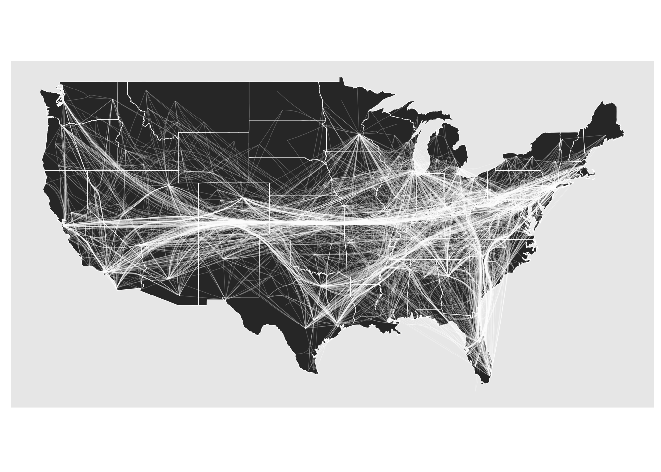
If the above stated caveats have made you skeptic, ggraph also provides an alternative bundling technique that tackles both of them. The edge path bundling algorithm doesn’t use any attracting forces when bundling. Instead it directs edges through their shortest path on an increasingly sparse version of the input graph. This, again, results in bundling, but this time the topology of the graph is being used so the bundles should to a larger degree make sense. It is also much faster to compute.
ggraph(gr, x = longitude, y = latitude) +
  geom_polygon(aes(long, lat, group = group), states, color = 'white', linewidth = 0.2) +
  coord_sf(crs = 'NAD83', default_crs = sf::st_crs(4326)) +
  geom_edge_bundle_path(color = 'white', width = 0.05)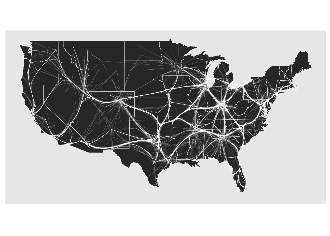
In every way an improvement. However, remember that, just like with layouts, there is no single right answer when it comes to edge bundling. You are introducing a bias to the representation and trying out different approaches is always a good idea.
The last bundling technique is very quick and dirty and a home invention of mine. It works much like the edge path bundling but instead of gradually removing edges from the graph where the shortest path is searched for, they are all found in the minimal spanning tree so it can be done in one go. This makes it the most performant of the three but suffers from forcing a tree-like structure onto the topology that the edges follows. It usually also requires a higher max_distortion setting since the minimal spanning tree forces edges on a larger detour.
ggraph(gr, x = longitude, y = latitude) +
  geom_polygon(aes(long, lat, group = group), states, color = 'white', linewidth = 0.2) +
  coord_sf(crs = 'NAD83', default_crs = sf::st_crs(4326)) +
  geom_edge_bundle_minimal(color = 'white', width = 0.05, max_distortion = 10)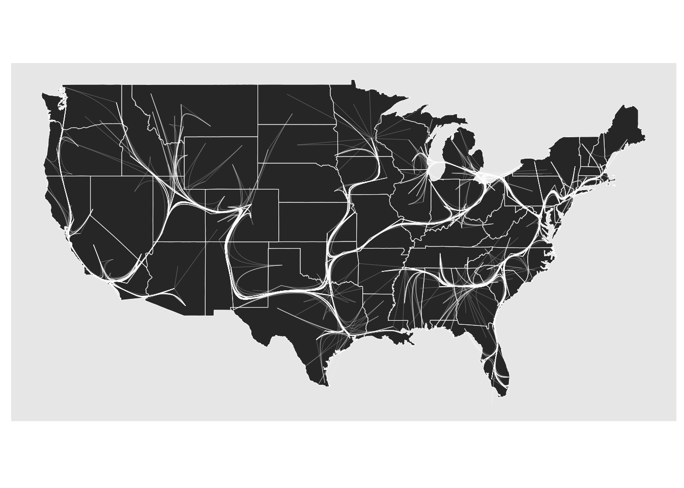
All in all, the edge bundling support has been greatly enhanced. I’d still like to add a technique that better splits out edges going in opposite direction but that will be for another release. Edge path bundling does treat directed graphs differently since the shortest path is direction dependent but there are also other techniques that are worth exploring
# This network doesn't really make sense to view as directed but we do it anyway
# to show the difference in output
gr <- gr |> convert(to_directed)
ggraph(gr, x = longitude, y = latitude) +
  geom_polygon(aes(long, lat, group = group), states, color = 'white', linewidth = 0.2) +
  coord_sf(crs = 'NAD83', default_crs = sf::st_crs(4326)) +
  geom_edge_bundle_path(color = 'white', width = 0.05)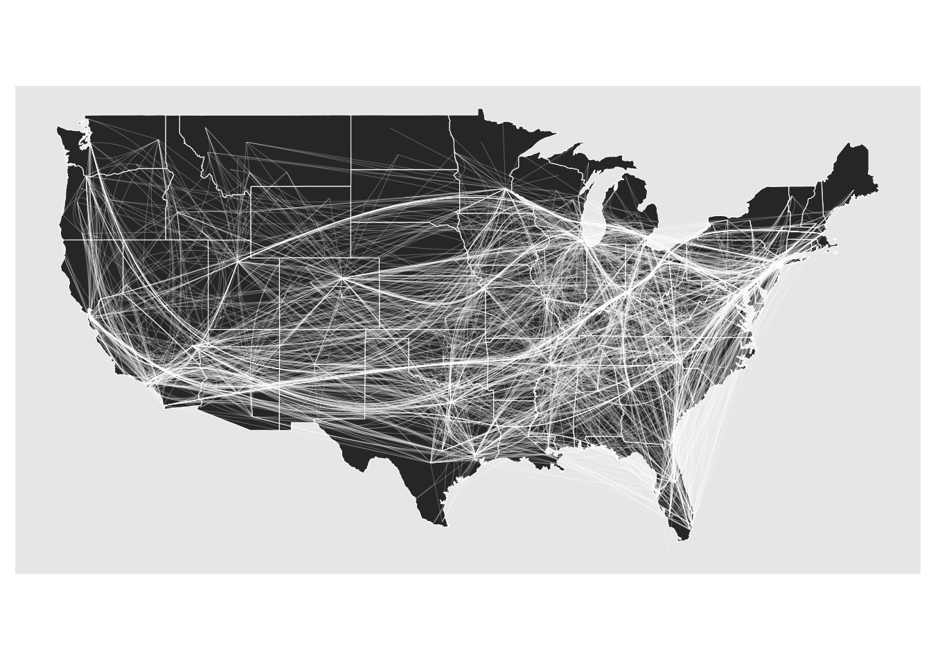
That’s about it. The release of course also includes numerous bug fixes, which was the whole reason why I started working on it in the first place. A lot of the new features presented couldn’t have happened without the work of David Schoch who has made great contributions to the network support in R and in tidygraph and ggraph in particular. Also a big thanks to the people working on sfnetworks and Lorena Crespo in particular for adding support in ggraph.